1.1. OPENMARU Observability Product Overview
A zero-instrumentation unified observability platform for Kubernetes
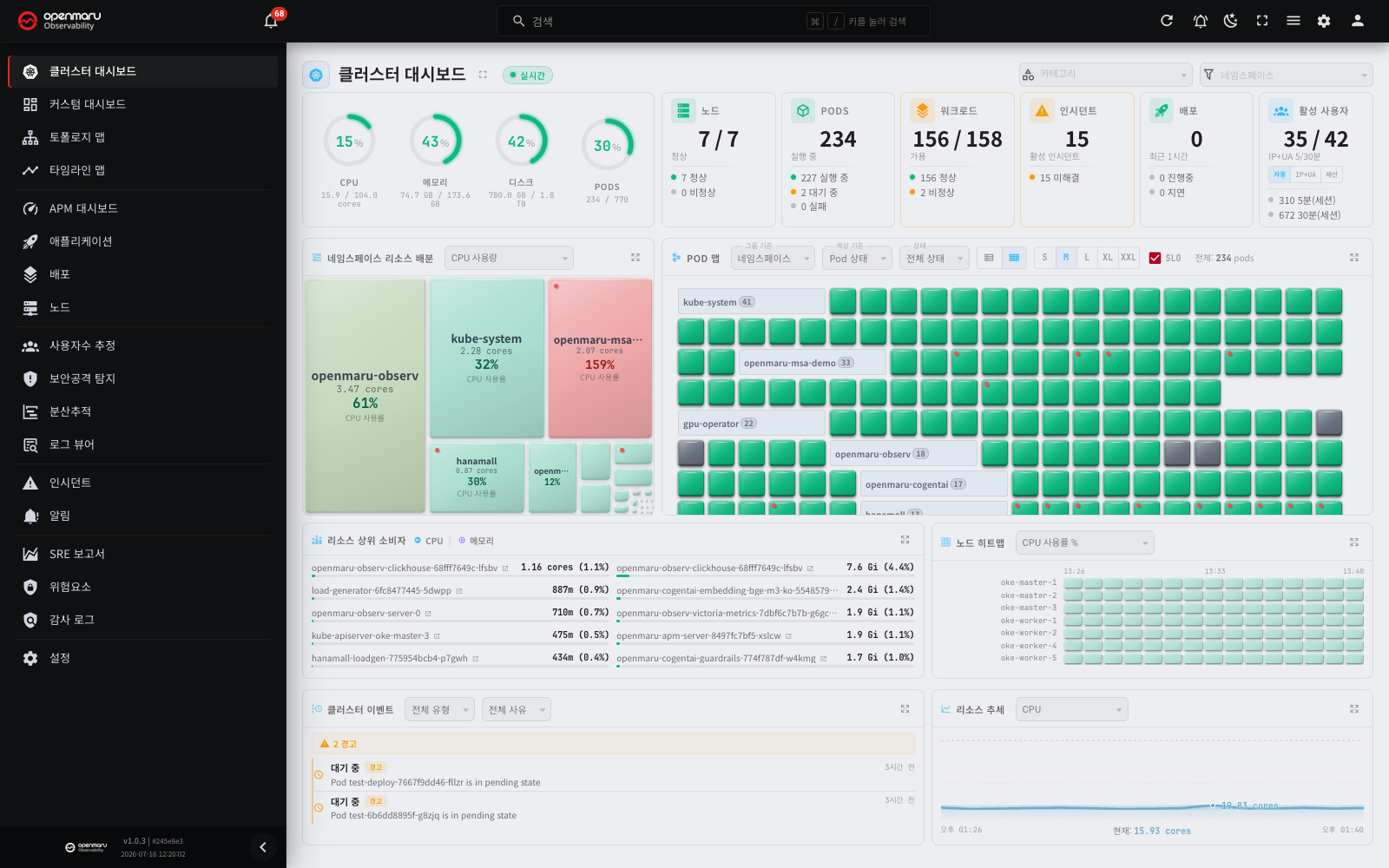
Product overview
OPENMARU Observability is an end-to-end observability solution for Kubernetes and cloud-native applications. Built on eBPF, it collects metrics, logs, traces and profiles automatically without modifying application code, so that operations teams can see the whole system at once.
Unlike conventional monitoring tools, it needs no SDK insertion and no code instrumentation. It works the moment it is installed and gives 100% visibility across your infrastructure, including legacy services.
Observability for practising SRE
SRE (Site Reliability Engineering) applies software engineering principles to system operations so that reliability — availability and performance — is managed with metrics, targets and automation rather than intuition. OPENMARU Observability goes beyond plain monitoring and backs that methodology with data. On top of data collected without any code instrumentation, it provides SLOs and error budgets, the golden signals (latency, traffic, errors, saturation), root cause analysis (RCA) and capacity forecasting, so teams can manage reliability in numbers and reduce toil.
The SRE report chapter covers what SRE is, its benefits and focus areas, and maps each SRE activity to the product features that support it.
Key strengths
1. Zero-instrumentation observability — install and start
Conventional APM (Application Performance Monitoring) tools and OpenTelemetry require language-specific instrumentation work.
- Java: you must add a
-javaagentoption when starting the JVM (for examplejava -javaagent:/path/to/agent.jar -jar app.jar). Every major APM tool and the OpenTelemetry Java Agent require this. - Python: you install the APM agent package with
pip installand either add a wrapper to the application start command (opentelemetry-instrument python app.py) or modify code for framework integration. - Node.js: after installing the instrumentation package, the agent must start before the application loads any other dependency (
--importflag orrequireinjection). With bundlers such as Webpack, compatibility problems can stop the agent from working. - Go: automatic instrumentation is limited, so you import the OpenTelemetry SDK into your source and write the code that creates traces and metrics.
- .NET: you install the agent NuGet package and set environment variables, or add the SDK to your source.
OPENMARU Observability needs none of this. It uses eBPF in the Linux kernel to collect telemetry at kernel level.
- No code changes: metrics, logs, traces and profiles are collected without changing a single line of application source, adding JVM options or installing agent packages.
- Language and framework agnostic: Java, Go, Python, Node.js, .NET — every stack is monitored the same way. There is no per-language agent to install or maintain.
- Legacy services included: third-party and legacy services that cannot be instrumented with OpenTelemetry are still traced through eBPF.
- Automatic protocol detection: HTTP, PostgreSQL, MySQL, Redis, MongoDB, Memcached, Kafka, Cassandra, RabbitMQ, ClickHouse, ZooKeeper and DNS are recognised and traced automatically, with no code change.
Impact: instrumentation work — per-service agent installation, JVM option changes, SDK code insertion — disappears. Development effort is saved and you get visibility across the whole system from day one.
2. 100% system coverage — no blind spots
Traditional monitoring can only observe instrumented services, which leaves blind spots. OPENMARU Observability traces network communication for every container at kernel level, so it builds a complete service map automatically without a service mesh.
- Automatic service map: dependencies and traffic flows between services are visualised in real time.
- TCP connection tracing: all service-to-service communication is detected automatically at kernel level.
- Node agent collection: deployed as a DaemonSet, it covers every node in the cluster automatically.
Impact: no service is "missing from monitoring" — you see the true state of the whole infrastructure.
3. Actionable insight — problems identified automatically
OPENMARU Observability does more than visualise data. More than 80 predefined inspections identify problems automatically, so the system detects an anomaly and tells you before an operator has to read a dashboard.
- Automatic inspection: predefined checks for CPU, memory, network, storage, databases and other areas run automatically.
- SLO-based alerting: availability and response time are monitored against SLOs (Service Level Objectives), and critical or warning alerts are raised according to how fast the error budget is burning.
- Incident root cause analysis (RCA): when an incident occurs, the causing service, the propagation path and the causal timeline are analysed automatically.
- Deployment regression detection: performance drops and error increases after a new release are detected by automatic comparison.
Impact: shortens MTTR (Mean Time to Resolution) — from noticing a failure to knowing its cause.
4. Unified observability — every signal on one platform
Metrics, logs, traces and profiles are brought together on a single platform, so you can follow a problem without switching tools.
| Data type | What you get |
|---|---|
| Metrics | Real-time time-series for CPU, memory, network, disk, GPU and more |
| Logs | Automatic pattern extraction, severity classification |
| Traces | Distributed trace heatmap, error analysis, response-time flame graph comparison |
| Profiling | Continuous CPU profiling, line-level performance analysis |
- Automatic log pattern extraction: log messages are clustered automatically so repeating patterns become visible.
- Flame graph comparison: compare the CPU profile of one period against another to find the cause of a slowdown at code level.
Custom dashboards let you combine that data however you like. Alongside metrics (PromQL) you can put logs, audit logs, security events, APM spans and user counts on one screen, drawn as time-series charts, single values, tables, bar lists, heatmaps or realtime widgets. Start from a ready-made template, clone it and edit, or export it as JSON to move it to another environment. See 3.2 Custom dashboards.
Impact: no need to run a separate log analysis tool, APM tool and profiler — one platform covers all of it.
5. Very low performance impact
The eBPF agent runs on the safe execution model the kernel guarantees, so it can be used in production with confidence.
- Low impact under load: even at high request rates, enabling the agent changes application response time only marginally.
- Low agent resource usage: because eBPF processes data inside the kernel, it adds no load to the application's request path, and the agent's own CPU and memory usage stays low. (For default resource settings, see the resource requirements table in the Installation chapter.)
- Kernel safety (read-only observation): an eBPF program is loaded and run only after it passes the Linux kernel verifier — infinite loops and invalid memory access are rejected at load time. The agent operates in read-only observation mode over kernel, network and system call events; it does not modify kernel code or application memory and injects no code, so it does not affect how the kernel or your applications behave.
- Safe under data overload: if CPU resources run short, some statistics may be dropped, but application performance itself is not affected.
Impact: you can add observability to production workloads without a performance penalty.
6. Kubernetes-native design
The architecture is built for Kubernetes, and a Helm chart makes deployment and operation straightforward.
- One-command Helm deployment: a single Helm command installs the whole stack — server, UI, agents and storage.
- Automatic resource discovery: Pods, Services, Deployments, StatefulSets and more are discovered through the Kubernetes API.
- Wide environment support: self-managed clusters, EKS, GKE, AKS, OKE, OpenShift, OPENMARU COP, K3s and MicroK8s.
Impact: designed for Kubernetes operations, so it can be adopted quickly with no separate infrastructure setup.
CogentAI — AI-driven intelligent analysis
OPENMARU Observability provides real-time, AI-driven analysis through CogentAI. On the chart, log and audit log screens, a single AI icon requests analysis immediately, and you can follow up in natural language for a deeper look.
One-click AI analysis
Every analysis starts by clicking the AI analysis button on the screen you are already looking at. CogentAI analyses the data in front of you with no configuration and no query to write.
Chart analysis
Request AI analysis on a time-series chart and CogentAI identifies anomalous patterns in the metric data and tells you what to do about a warning right away. It offers relevant kubectl commands and concrete remediation steps, and for events that recur it concentrates on root cause analysis.
Log analysis
Request AI analysis on a log message and CogentAI interprets what the log means. It explains each field — timestamp, log level, class, message body — and for WARN, ERROR and CRITICAL entries it works out the cause of the error and proposes a fix. For INFO and DEBUG entries that describe normal operation, it explains the meaning without recommending unnecessary action.
Audit log analysis
Audit logs are analysed from a security point of view.
- Kubernetes audit logs: analysed against Kubernetes RBAC policy and security best practice. Unusual access patterns and privilege escalation attempts are identified, with recommendations for hardening.
- OS audit logs: analysed against system security best practice to identify unusual process execution or file access, with recommendations for hardening.
Insight grounded in official Kubernetes documentation
CogentAI bases its analysis on the official Kubernetes documentation and best practice. It proposes solutions built purely on Kubernetes' own capabilities and kubectl commands, so the insight is practical and can be applied to a live environment straight away.
Advanced analytics
Beyond basic monitoring, OPENMARU Observability offers advanced analytics so that operations teams can anticipate problems and find the root cause of a failure automatically.
Forecast — time-series prediction
Predict future trends from a chart with one click, and prepare for resource exhaustion or performance degradation before it happens.
- One-click forecast: click the forecast button on any time-series chart and the future trend is predicted immediately from historical data.
- Five algorithms: Auto (automatic selection), Holt-Winters, Linear, ARIMA and SARIMA. In Auto mode the best algorithm is chosen according to the characteristics of the data.
- Confidence interval visualisation: the forecast is overlaid on the existing chart as a dashed line with a confidence band, so the range of uncertainty is visible.
- Flexible horizon: choose 10 minutes, 30 minutes, 1 hour, 2 hours, 3 hours, 6 hours or 12 hours.
- Automatic fallback: if forecast accuracy is low, the system switches algorithms automatically to keep the result stable (SARIMA → ARIMA → Holt-Winters → Linear).
Example: run a forecast on a CPU usage chart to see whether you will hit a resource limit in the next few hours (up to 12), and plan scaling accordingly.
Anomaly detection
Outliers that fall outside the normal range are detected automatically in time-series data, catching subtle signs that manual monitoring would miss.
- On-demand anomaly detection: click the anomaly detection button on a chart to analyse that metric immediately.
- Four detection algorithms: Z-Score (statistical deviation), IQR (interquartile range), Isolation Forest (ML-based) and RCF (Random Cut Forest).
- Expected-range band: the normal range is drawn as a band and the intervals outside it are highlighted, so anomalies stand out at a glance.
- Sensitivity control: adjust detection sensitivity to set the anomaly threshold that suits your environment.
- Direction: detect upward anomalies (spikes), downward anomalies (drops) or both.
Example: run anomaly detection on a network response time chart to identify automatically the periods where the response-time pattern differed from usual, and start investigating from there.
Deployment Timeline
Deployment events and incidents are visualised together on one time axis, so the relationship between a release and a failure is immediately clear.
- Combined event timeline: deployments (point events) and incidents (interval events) are shown as a two-lane swimlane on a single time axis. Deployments appear as point markers, incidents as bars from start to end.
- Time correlation: "did an incident follow this deployment?" is answerable at a glance. Deployments and incidents are compared visually by how close they are in time.
- Event density management: dense events are clustered automatically and shown with a count badge. Clusters are recalculated as you change zoom level.
- Brush-to-zoom: drag across the timeline to zoom into a period and explore the events in detail.
- One-click drill-down: click an event on the timeline to jump straight to the application detail view for that deployment, or to the incident detail view.
Example: when investigating an incident that happened overnight, identify from the timeline the deployment that ran just before it and check what that release changed.
User estimation
The number of active users in real time is estimated from the HTTP traffic the agent already collects. No tracking code in the application, no browser cookie of ours, no external analytics tool.
- Two estimation methods: counted by session where a session cookie exists, otherwise by IP + User-Agent. Chosen automatically, or set by hand
- DAU / WAU / MAU: daily, weekly and monthly active users
- Regional distribution: country and region breakdown on a map, from the source IP
- User activity report: download the active-user trend for a period as a report
Example: active users drop sharply right after a deployment, which points at a feature regression or a broken login. It catches the case where server metrics look fine but users are going away. See 7.1 User estimation.
RCA (Root Cause Analysis)
When an incident occurs, the dependency graph is traversed automatically to trace the root cause and visualise how the impact propagated. It answers "why did this happen?" without manual analysis.
- Two-stage automatic analysis: first a structural analysis traverses the dependency graph and compares telemetry, then the findings are summarised with proposed fixes. The structural stage uses a deterministic method, so the result is reproducible and explainable.
- SLI heatmap: response time and error rate during the incident are shown as a heatmap. Select an area of the chart to drill down into a specific time window.
- Propagation map: starting from the root cause service, the path the impact travelled is drawn as a multi-level service graph. Each service is coloured by state (normal, warning, critical).
- Hypothesis tree: possible causes are presented as a hierarchical tree. Each hypothesis carries a sparkline, log patterns and related metrics so you can check the evidence.
- Causal timeline: the order of events from cause to effect is laid out on a timeline so the causal chain can be followed.
- Inspection-based analysis: predefined checks for CPU, memory, network, storage, databases and other areas identify the problem automatically.
Example: when an SLO violation incident is raised on the payment service, the RCA tab identifies automatically that the root cause was lock waiting in a downstream database service, and shows the path by which the impact spread from payment to orders to the front end.
Compared with conventional monitoring tools
| Aspect | Conventional APM / monitoring | OPENMARU Observability |
|---|---|---|
| Instrumentation | Per-language agent install, JVM options, SDK code insertion | Zero instrumentation with eBPF |
| Coverage | Only instrumented services | Every service, automatically (100%) |
| Service map | Needs a service mesh or manual configuration | Generated automatically (TCP connection tracing) |
| Time to adopt | Weeks to months (per-service instrumentation) | Hours (works as soon as Helm install finishes) |
| Legacy services | Blind spots where instrumentation is impossible | Traced through eBPF, legacy included |
| Performance impact | SDK overhead | Processed outside the application path (in kernel), impact marginal |
| Problem identification | Manual dashboard analysis | 80+ automatic inspections |
| Unified data | Separate metric, log and trace tools | One platform |
| AI-driven analysis | Separate tool integration, or none | CogentAI one-click analysis built in |
| Time-series forecasting | Needs a separate ML tool | One-click forecast in the chart (5 algorithms) |
| Anomaly detection | Manual threshold setting | On-demand anomaly detection (4 algorithms) |
| Root cause analysis | Manual log and metric analysis | Automatic RCA (dependency graph traversal + hypothesis tree) |
| Deployment–failure correlation | Manual comparison in a separate tool | Visual correlation on a combined timeline |
Business impact
Better operational efficiency
- Shorter MTTR: automated incident RCA shortens the time it takes to find the cause of a failure. The hypothesis tree and propagation map make even complex microservice failures analysable in a systematic way.
- Immediate AI analysis: CogentAI performs one-click AI analysis on charts, logs and audit logs, reducing the analysis load on operators and speeding up response.
- Preventing failures: SLO-based error budget monitoring combined with forecasting detects resource exhaustion and performance degradation before they bite.
- Safer deployments: the deployment timeline shows the time correlation between a release and an incident immediately, and performance regression before and after a release is compared automatically.
- Early detection of anomalies: anomaly detection identifies subtle patterns before a threshold is reached, so you can act first.
Lower cost
- Tool consolidation: metrics, logs, traces and profiles on one platform reduce licence costs for multiple tools.
- No instrumentation development cost: the development effort spent inserting and maintaining per-service SDKs disappears.
- Lower log storage cost: automatic log pattern extraction clusters repeating messages by template, and ClickHouse's columnar compression (several to tens of times, depending on the data) cuts storage usage.
- Resource optimisation: cloud cost analysis identifies idle resources and over-provisioning.
Higher development productivity
- Code-level performance analysis: continuous profiling traces bottlenecks down to a specific line of code.
- Automatic distributed trace analysis: thousands of traces are analysed automatically, with error causes and slow segments summarised.
- Faster developer onboarding: the service map and dependency visualisation help new team members understand the system quickly.
Use cases
Case 1: tracing a microservice failure
Situation: a system built from dozens of microservices shows intermittent response delays, but it is hard to tell which service is responsible.
With OPENMARU Observability:
- Check dependencies and traffic state between services at a glance on the Topology Map.
- Identify visually, on the distributed trace heatmap, the periods and requests where the delay occurs.
- Select the traces in that interval and the system analyses all of them automatically to produce a latency flame graph, showing which call in which service is the bottleneck.
- Use incident RCA to find the root cause service and the propagation path automatically.
Result: failure analysis that used to take hours completes in minutes.
Case 2: detecting performance regression after a release
Situation: after deploying a new version, reports come in that some APIs have become slower.
With OPENMARU Observability:
- Confirm when the service was deployed from the deployment history.
- Visualise the time correlation between deployment events and incidents on the Timeline Map.
- Compare CPU, memory and response time before and after the release as a chart overlay in application detail metrics.
- In profiling comparison mode, compare the CPU flame graphs of the old and new versions; the functions that regressed are marked in red.
Result: a deployment regression is detected immediately and its cause found at code level, so you can roll back or fix quickly.
Case 3: diagnosing a database bottleneck
Situation: response times have slowed across the service and the database is suspected.
With OPENMARU Observability:
- Check the database connections the service depends on from the service map.
- Look at the database query spans captured automatically, with no code change, in eBPF-based tracing.
- Analyse slow queries, lock waits and connection pool state in the database agent metrics.
- See how database error patterns are trending in log patterns.
Result: you learn exactly which query consumes the most resources and which queries to optimise.
Case 4: optimising Kubernetes cluster resources
Situation: cloud cost is rising but it is hard to tell which service is over-using resources.
With OPENMARU Observability:
- Check the gap between cluster-wide CPU/memory allocation and actual usage on the Cluster Dashboard.
- See how resources are distributed on the per-namespace resource treemap.
- Identify nodes with a lot of idle capacity in node detail.
- Find services whose actual usage is far below their requests in per-application metrics, and rebalance.
Result: over-provisioned resources are identified and cloud cost comes down.
Case 5: detecting security attacks in real time
Situation: a web service exposed to the internet needs SQL injection, XSS and similar attack attempts detected and handled in real time.
With OPENMARU Observability:
- On the Attack Detection screen, HTTP traffic collected by eBPF is analysed to detect SQL injection, XSS, RCE and other attack patterns in real time.
- Detected attacks are classified by severity (HIGH, MEDIUM, LOW), with the top attacking IPs and the targeted applications listed.
- Trends per attack type and KPIs show when an abnormal spike began.
- Real-time alerts notify you of serious attacks immediately, and false positives are excluded with an IP allowlist.
Result: attacks are detected at kernel level in real time and handled quickly, with no application code change and no separate WAF.
Case 6: real-time error detection from logs
Situation: important errors must not be missed among the large volume of logs produced by dozens of services.
With OPENMARU Observability:
- Apply a severity filter (ERROR, WARN) in the Log Viewer to see only error logs.
- Use log pattern mode to cluster repeating error messages automatically and group them by error type.
- See when a particular error pattern started to spike on its trend chart.
- Analyse what an error log means and how to resolve it with CogentAI.
Result: key errors are classified automatically out of a large log volume, so causes are found quickly.
Who it is for
OPENMARU Observability suits organisations that:
- operate Kubernetes-based infrastructure and need unified monitoring
- have adopted, or are moving to, a microservice architecture
- find the instrumentation cost of existing APM tools a burden
- need visibility with no blind spots across a hybrid environment that includes legacy services
- are adopting an SRE/DevOps culture and want SLO-based operations
- work in an enterprise environment with security compliance requirements
- want to improve operational efficiency through AI-driven automation
System requirements
| Item | Requirement |
|---|---|
| Kubernetes | 1.23 or later (self-managed, EKS, GKE, AKS, OKE, OpenShift, OPENMARU COP, K3s, MicroK8s) |
| Linux kernel | 4.16 or later (eBPF support) |
| Deployment tool | Helm 3.x or later |
| Storage | PostgreSQL 16.8 (metadata), VictoriaMetrics 1.145.0 (metrics), ClickHouse 26.5.1 (logs/traces) |
| Container runtime | Docker, Containerd, CRI-O |
Note: every component is deployed automatically by the Helm chart. PostgreSQL, VictoriaMetrics and ClickHouse are included in the chart.
Caution: Docker-in-Docker environments (such as MiniKube) and WSL1 (Windows Subsystem for Linux) are not supported because of eBPF limitations.
Next steps
If the product interests you, the following documents will help you try it yourself.
- Quick start guide — from installation to your first data
- Installation guide — the full guide for a production install
- Dashboard — start monitoring the state of your cluster
Related documents
- Common chart guide — reading time-series charts, forecasting, anomaly detection
- Topology map — visualising dependencies between services
- Applications — per-application monitoring in detail
- Distributed tracing — exploring and analysing distributed traces
- Incidents — SLO violation incidents and root cause analysis
- Settings — alerts, inspection conditions, user management